Approaches to Consider for Site-Specific Field Mapping
Overview
Traditional agricultural practices—such as considering one parcel (10–50 acres) as one unit when determining soil fertility status—overlook the spatial and temporal variability of nutrients within the farm unit. Treating an entire field as a single unit may lead to over-fertilization or under-fertilization of areas due to differences in the buildup of nutrients in the soil. Figures 1, 2, and 3 demonstrate how soil pH, soil organic matter, and soil textures can vary across a 50-acre parcel.
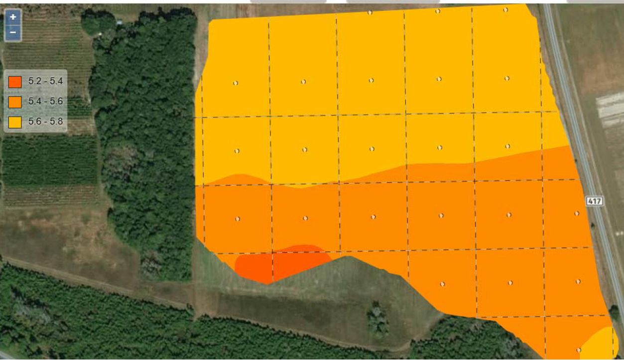
Credit: C. Barrett, UF/IFAS
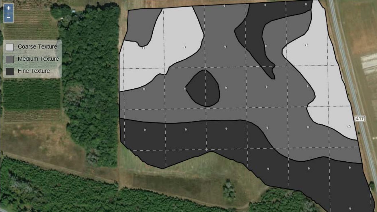
Credit: C. Barrett, UF/IFAS
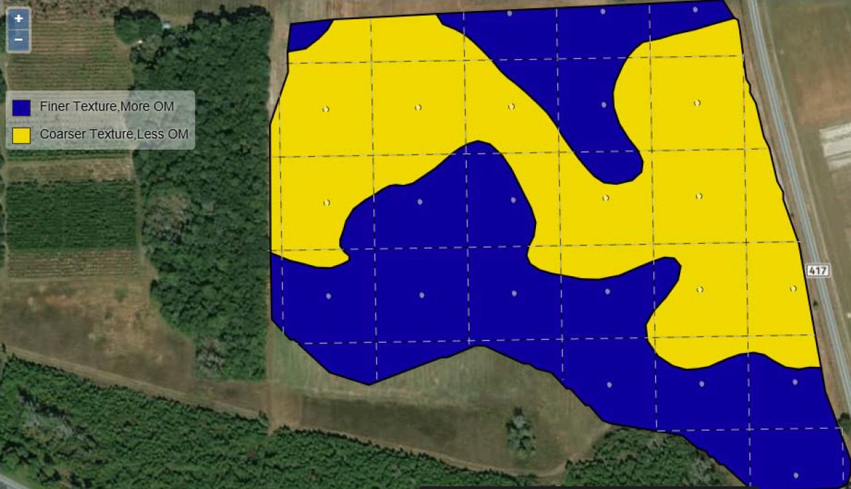
Credit: C. Barrett, UF/IFAS
To meet rising food and fiber needs, researchers have been developing high-yielding crop varieties that need more nutrition, resulting in higher fertilizer applications by farmers; crop hybrids remove more nutrients from the soil than the older varieties from which several land grant universities based nutrient recommendations (Bruuslema et al., 2012). The advent of improved germplasm has thus rendered several nutrient recommendations impractical, and, following these recommendations, farmers have applied nutrients above the recommended limit. 240 lb. of nutrients per acre should not be applied to corn as “recommended,” nor should 60 lb. of nutrients per acre to cotton. Excessive fertilizer use can lead to environmental issues if poorly managed. Due to limited resources, conducting field trials every 5 to 10 years to update nutrient recommendations may not be feasible. Therefore, site-specific farming could be a more feasible way to increase farm income, minimize environmental issues, and provide a more sustainable production system (Robertson et al. 2009; Swenson and Haugen 2009; Griffin et al. 2008). This publication explains soil-based site-specific farming basics for agriculture Extension agents, allied industry consultants, researchers, and farmers.
Soil-Based Site-Specific Management
Variability in soil properties within a field can cause uneven crop production; therefore, a soil assessment is required to gauge variation before crop planting or at planting. The difference in soil properties could be apparent through grid/zone soil sampling, previous year’s yield maps, etc. Variability in soil properties is generally caused by differences in topography, soil texture, organic matter, soil moisture, soil color, and sand grains (Mann et al. 2018). Site-specific management accounts for variability in soil, assembles information, and modifies input requirements.
Adopting a Soil-Based Site-Specific Approach
Most farmers perceive site-specific farming tools as expensive and difficult to use (Ghatrehsamani et al. 2018). However, as studies at several north-central and southeastern land-grant institutions have shown, site-specific tools may result in lower production costs, higher yields, more net income, and less environmental damage (Franzen 2018). For example, electrical conductivity (EC) maps, zone/grid soil sampling maps, ground-based active optical sensors, moisture meters, and climatic data have been successfully calibrated in North Dakota, Oklahoma, Nebraska, Missouri, and North Carolina for side-dress nitrogen application in corn. It is important to note that farmers from these states have adopted zone and grid soil-sampling techniques to detect low- and high-fertility areas for variable-rate fertilizer applications before or at planting. However, the above-mentioned tools were calibrated using intensive research in those states; therefore, they may not be directly applicable in Florida.
Site-specific farming involves farmers thinking ahead and in a different way compared with conventional farm practices. It involves critical steps that must be followed accurately. Typically, there are three fundamental steps to using soil-based site-specific management:
- Create a field variability map with prescription capability using:
- EC maps,
- Grid/zone soil sampling maps,
- Soil moisture sensor maps,
- Soil nutrient sensor maps,
- Soil drone imagery (e.g., development of soil organic matter maps), and/or
- Normalized Difference Vegetative Index (NDVI) maps
2. Modify/procure tools (e.g., variable-rate applicators or location and speed sensors like GPS) to implement prescriptive management according to field and yield maps.
3. Quantify the results for comparison.
Create a Prescription-Capable Field Map
Geographic information systems (GIS) are tools available to develop maps that show the soil nutrient variability within certain land areas. The yield, field, or EC maps, help determine variable-rate applications for site-specific management. A GIS can compile data using several approaches (e.g., soil sampling, satellite data) to visualize a specific area's soil pH value and nutrient content.
Every field mapping technique has advantages and disadvantages, from cost-effectiveness to variability determination. Prescription maps are most often created from EC measurements (as Floridian prescription maps for corn are) and grid soil sampling; expensive in the early 2000’s, EC maps have recently become cheaper to manufacture and, thus, buy.
The EC mapping tools like VERIS (model: MSP3-Tractor Series from Veris technologies) can help one understand a field’s soil texture and organic matter patterns. For example, in Figure 4, three types of soil textures can be seen in an approximately 50-acre parcel in Live Oak, FL. Treating this whole field as one unit may result in over- and under-application of fertilizers and non-uniform yield patterns. Loss of nitrogen (N), phosphorus (P), and potassium (K) fertilizers may also occur with over-fertilization. Based on this EC map, this field has the potential for N loss through volatilization as nitrous oxide or N2 gas (in fine-textured soils when saturated with water) or by leaching as nitrate (in medium and coarse-textured soils). If a farmer applies a relatively higher proportion of the total required N fertilizer at planting (about 100 lb. N/acre on potatoes or about 50–80 lb. N/acre on corn) and crop yield thereafter diminishes, then these losses are likely due to potential leaching.
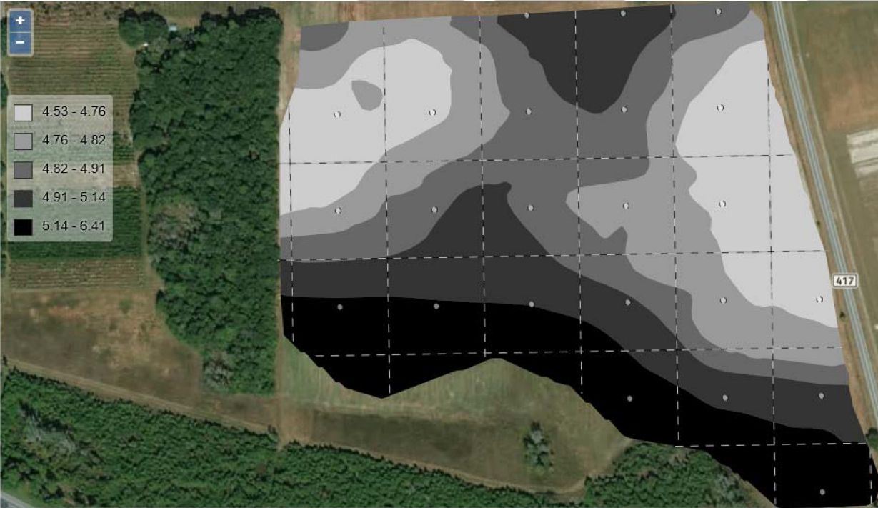
Credit: C. Barrett, UF/IFAS
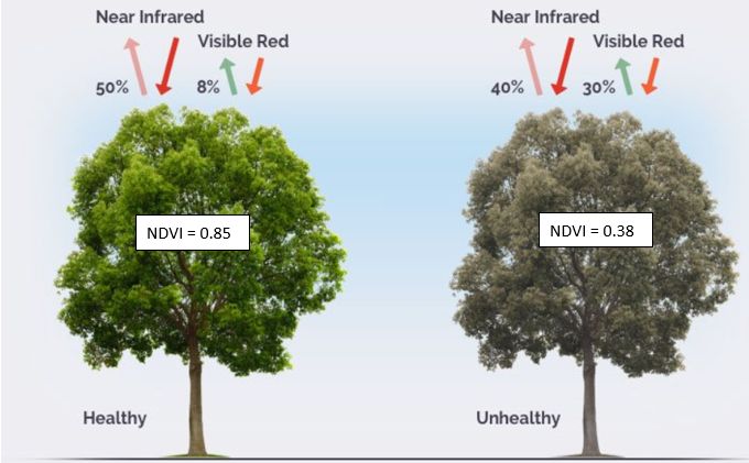
The NDVI is a ratio of the spectral reflectance (i.e., the energy that a surface reflects at a specific wavelength) at red and near-infrared (NIR) wavelengths (Equation 1). The NDVI has long been used to predict plant health and crop yield (Costa et al. 2020). Researchers have developed several algorithms using NDVI to predict the required N for many crops (Ransom et al. 2020; Sharma and Bali 2017). As shown in Figure 5, the NDVI value of non-green or pale green foliage is lower than that of green foliage. The low NDVI from pale green foliage is due to the more visible wavelength reflection and, consequently, less light absorption. NDVI measurements (which have a maximum of 1 and a minimum of 0 for vegetation) provide insight into the relative health of the crop.
NDVI = (NIR-Red)/(NIR) + (Red)
Credit: NASA
NDVI maps are another way to determine the in-field spatial variability of crop yield. Figure 6 shows an NDVI map of an approximately 3-acre parcel planted with corn at the 8-leaf growth stage. The corn foliage varies between 0.39 and 0.66 NDVI. A higher NDVI value (close to 1) in a field can signify better crop health. In this example, if the 0.66 NDVI is close to the best possible NDVI from the corn foliage in that area, an NDVI map could help identify areas with poor crop health; and if there is an available algorithm to relate the poor health with N, then the required N for optimum yield could be estimated using the NDVI maps. Dr. Yiannis Ampatzidis has developed a commercially available citrus NDVI mapping system for citrus growers. This NDVI mapping system identifies the tree canopy color or structure and guides farmers in its management. Refer to this PowerPoint for more information: https://swfrec.ifas.ufl.edu/docs/pdf/nat-res-econ/resources/2019-05-16-W4-Ampatzidis.pdf.
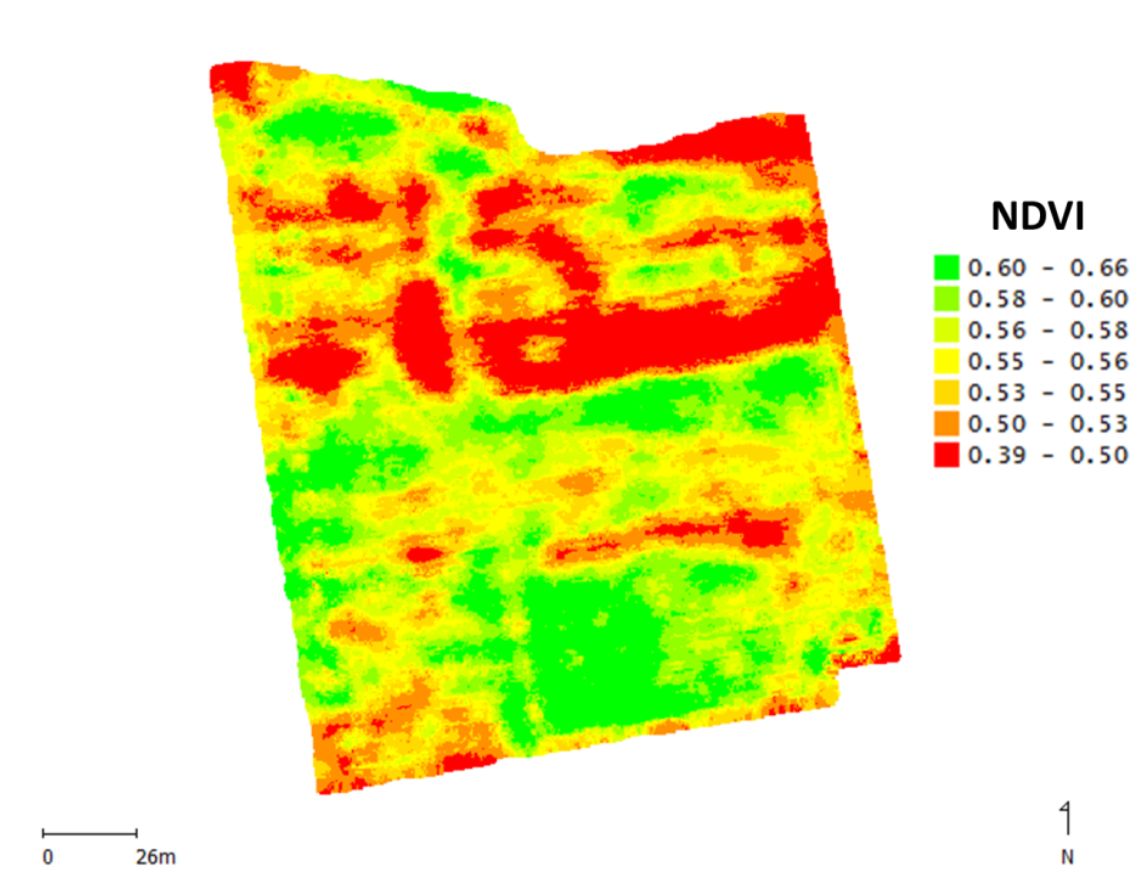
Credit: Povh, Fabrício (2014)
Modify/Procure the Tools to Apply the Prescription According to the Maps
Know your Location
GPS technology is well-established and in use throughout the world in many applications. It operates through a system of satellites developed by the U.S. Department of Defense that communicate signals to any receiver on Earth. By calculating the total time taken by the signal to reach a GPS receiver from multiple satellites, the receiver calculates its location in a three-dimensional position (latitude, longitude, and altitude) (Figure 6).
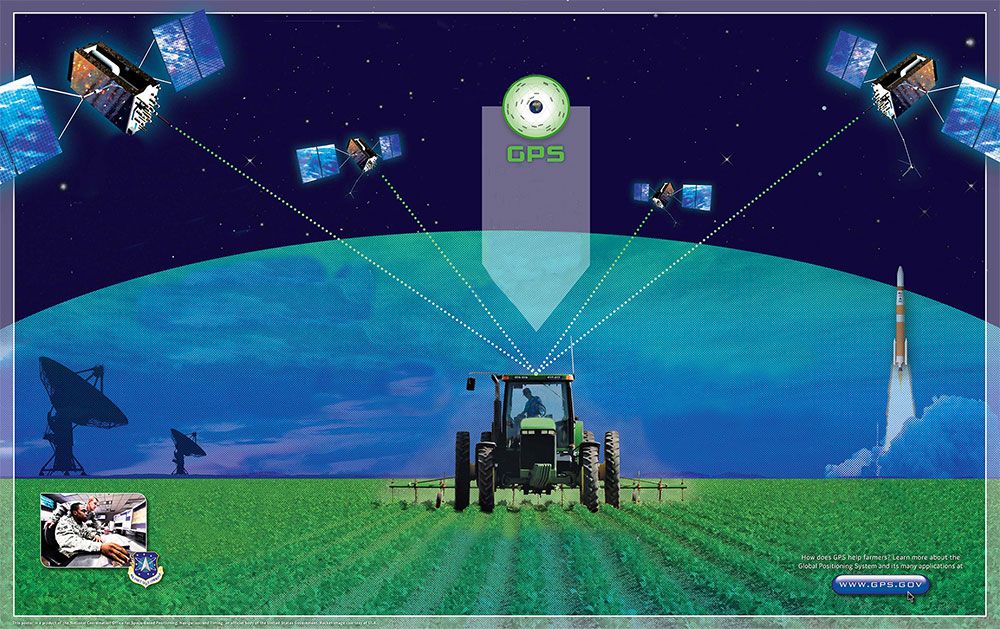
Credit: NASA
A GPS receiver, depending upon the capabilities, can find the position/location with an accuracy of a few inches to a few feet. Small errors in exact coordinates are possible, but “differential GPS” (DGPS) can improve positioning accuracies. Real-time kinematic (RTK) GPS-enabled tractor systems are also available in Florida. These systems can improve the precision of GPS data and are useful for horizontal and vertical applications. The RTK GPS system requires either an additional base station or a subscription to a company that provides base-tower signals for GPS receivers, such as commonly used cellular service providers. The use of GPS has many other benefits for site-specific applications. For example, it can be used for variable rate fertilizer application according to high/low yield potential areas of the field. It can help reduce double-cultivating and double applications of fertilizers and chemicals in a variable-rate nutrient application, and it can enable yield monitoring.
The GPS can be installed on older tractors, too. The tractor can be autosteered or manually controlled with GPS, but both could work with the previously discussed prescription maps. A technician from the tractor company could help the grower upload the variability maps (EC or NDVI) into the controller system of the tractor. Once the maps are loaded, the GPS will connect the map to real-time prescription (variable rate) applications. It is important to note that all these services come with several packages at different prices. The farmer should discuss all the options ahead of time because GPS subscription may also come with added features of NDVI mapping.
Variable-Rate application
After loading prescription maps to the GPS system, the farmer needs equipment to transform the information from map variability to input application. Most tractor dealerships have technology personnel that helps farmers patch up information from different sources. Several commercially available companies, including drones or soil mapping, help farmers to develop prescription maps. Several variable rates (VR) applicators are now available in the market, especially in the grain production system. Variable-rate controllers are available for need-based input applications; these controllers could be installed by modifying an old applicator. The technology personnel from the dealership could help farmers connect/talk the maps with the variable rate controller applicator software. These technologies can apply variable rate planting, fertilization, and insecticide in both granular and liquid forms. Although most controllers are compatible with various input/planting devices, checking with the manufacturer may be wise to determine the best option for a given situation. Most companies have technicians to help growers in selecting an appropriate tool for site-specific farming.
Quantify the Results for Comparison
One must also quantify their results to evaluate the variable rate applications. Most combines/harvesters are equipped with a yield monitor. With this tool, a farmer could generate yield maps and determine yield variability within a field. The yield maps could further determine prescription rates to improve the following year’s yield. The dealers/companies from which the farmer bought the combine provide services to map the yield and convert it to prescription maps for coming years. Yield maps show the variability of farm fields that could be linked back to EC or NDVI maps; yield maps also demonstrate additional factors across space and time, like weather or pest variability. Figure 8 is a corn yield variability map created by yield monitors. The corn yield varies from 2.3 bushels/acre in field edges to 294.7 bushels/acre in higher-producing areas. When edges are excluded from the data, yellow corn yield still varies from medium-green corn yield, the former 253.1 bu/acre and the latter 127.7 bu/acre. This could make a difference of $766 to $1519 in profits, assuming a corn bushel price of $6. These maps are developed using a yield monitor with a GPS; therefore, the yield monitor and related tools could help farmers better understand their fields and identify opportunities to fine-tune fertility management. This information can help one determine whether the low-producing area, 2.3 bushels/acre, can be improved, simplifying the decision-making process for the farmer; by checking the records of that parcel’s average, the farmer can determine whether their tested area could yield more if additional fertilizer is applied. This kind of information can teach farmers to not treat a parcel’s low-producing area the same way as its high-producing area.
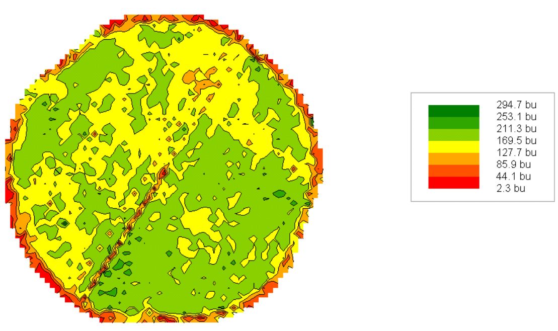
Credit: Joseph Berry, Innovative-GIS
Acknowledgment
We acknowledge Charles Barrett, former regional specialized Extension agent at the University of Florida, for providing the information on electrical conductivity.
References
2015. “UF/IFAS Evaluating Soil Mapping Technology for Variable Rate Applications.” UF/IFAS Blogs, May 29, 2015. https://blogs.ifas.ufl.edu/nfrec/2015/05/29/ufifas-evaluating-soil-mapping-technology-for-variable-rate-applications/
n.d. “Applying MapCalc Map Analysis Software.” http://www.innovativegis.com/basis/Senarios/VisYield_scenario.htm
Bruulsema, T.W., P. E. Fixen, and G. D. Sulewski. 2012. 4R Plant Nutrition Manual: A Manual for Improving the Management of Plant Nutrition. North American version. Norcross: International Plant Nutrition Institute. http://www.ipni.net/article/IPNI-3255.
Costa, L., L. Nunes, and Y. Ampatzidis. 2020. “A New Visible Band Index (vNDVI) for Estimating NDVI Values on RGB Images Utilizing Genetic Algorithms.” Computers and Electronics in Agriculture 172: 105334. https://doi.org/10.1016/j.compag.2020.105334
Franzen, D. W., L. K. Sharma, and H. Bu. 2014. “Active Optical Sensor Algorithms for Corn Yield Prediction and a Corn Side-Dress Nitrogen Rate Aid.” NDSU Extension Circular SF1176-5. https://www.ndsu.edu/fileadmin/soils.del/pdfs/sf1176-5.pdf
Franzen, D.W., L. K. Sharma, and H. Bu. 2014. “Site-Specific Farming-4: Economics and the Environment.” NDSU Extension Circular SF1176-4.
Ghatrehsamani, S., T. Wade, and Y. Ampatzidis. 2018. “The Adoption of Precision Agriculture Technologies by Florida Growers: A Comparison of 2005 and 2018 Survey Data.” XXX International Horticultural Congress IHC2018: VII Conference on Landscape and Urban Horticulture, IV Conference on 1279, 311–316. https://doi.org/10.17660/ActaHortic.2020.1279.44
Griffin, T., D. Lambert, and J. Lowenberg-DeBoer. 2008. “Economics of GPS Enabled Navigation Technologies.” In Proceedings of the 9th International Conference on Precision Agriculture, July 20–23, edited by R. Khosla. Denver.
EOS Data Analytics. “NDVI: Normalized Difference Vegitation Index.” Earth Observing System. https://eos.com/ndvi/
Pinheiro Povh, F., and W. Paula Gusmão dos Anjos. 2014. “Optical Sensors Applied in Agricultural Crops.” In Optical Sensors—New Developments and Practical Applications, edited by M. Yasin, S. W. Harun, and H. Arof. Rijeka: InTech. https://doi.org/10.5772/57145
Ransom, C. J., N. R. Kitchen, J. J. Camberato, P. R. Carter, R. B. Ferguson, F. G. Fernández, D. W. Franzen, et al. 2020. “Corn Nitrogen Rate Recommendation Tools’ Performance across Eight US Midwest Corn Belt States.” Agronomy Journal 112: 470–492. https://doi.org/10.1002/agj2.20035
Raun, W. R., J. B. Solie, M. L. Stone, K. L. Martin, K. W. Freeman, R. W. Mullen, H. Zhang, J. S. Schepers, and G. V. Johnson. 2007. “Optical Sensor-Based Algorithm for Crop Nitrogen Fertilization.” Communication Soil Science Plant Analysis 36: 2759–2781. https://doi.org/10.1080/00103620500303988
Robertson, M., P. Carberry, and L. Brennan. 2009. “Economic Benefits of Variable Rate Technology: Case Studies from Australian Grain Farms.” Crop and Pasture Science 60 (9). https://doi.org/10.1071/CP08342
Schepers, J.S., T. M. Blackmer, and D. D. Francis. 1992. “Predicting N Fertilizer Needs for Corn in Humid Regions: Using Chlorophyll Meters.” In Predicting N Fertilizer Needs for Corn in Humid Regions., edited by B. R. Bock and K. R. Kelley, 105–114. Muscle Shoals: National Fertilizer and Environmental Research Center.
Sharma, L.K., and S.K. Bali. 2016. “An Introduction to Using Site-Specific Farming to Manage Field Variability.” University of Maine Cooperative Extension, Bulletin #1080. https://extension.umaine.edu/publications/1080e/
Sharma, L. K., H. Bu, A. Denton, D. W. Franzen. 2015. “Active-Optical Sensors Using Red NDVI Compared to Red Edge NDVI for Prediction of Corn Grain Yield in North Dakota, USA.” Sensors 15 (11): 27832–27853. https://doi.org/10.3390/s151127832
Sharma, L.K., and D. W. Franzen. 2014. “Use of Corn Height to Improve the Relationship Between Active Optical Sensor Readings and Yield Estimates.” Precision Agriculture 15: 331–345. http://dx.doi.org/10.1007/s11119-013-9330-9
Sidhu S. S., D. L. Wright, S. George, and I. Small. 2021. “Nitrogen Calibration Strip: an On-Farm Tool to Further Reduce N Requirements in Cotton on an Integrated Crop-Livestock Rotation System.” Agronomy Journal 113: 3615–3627. https://doi.org/10.1002/agj2.20730
Small, I. M., and D. L. Wright. 2020. “Sustainability Aspects of Precision Agriculture for Row Crops in Florida and the Southeast United States: SSAGR184/AG186, Rev. 9/2020”. EDIS 2020 (5): 5. https://doi.org/10.32473/edis-ag186-2020
Swenson, A., and R. Haugen. 2009. “Projected 2009 Crop Budgets South Valley North Dakota.” NDSU Farm Management Planning Guide, North Dakota State University Extension. https://www.ndsu.edu/agriculture/sites/default/files/2021-10/sv2009.pdf

